Dynamical Downscaling of Coastal Dynamics for Two Extreme Storm Surge Events in Japan

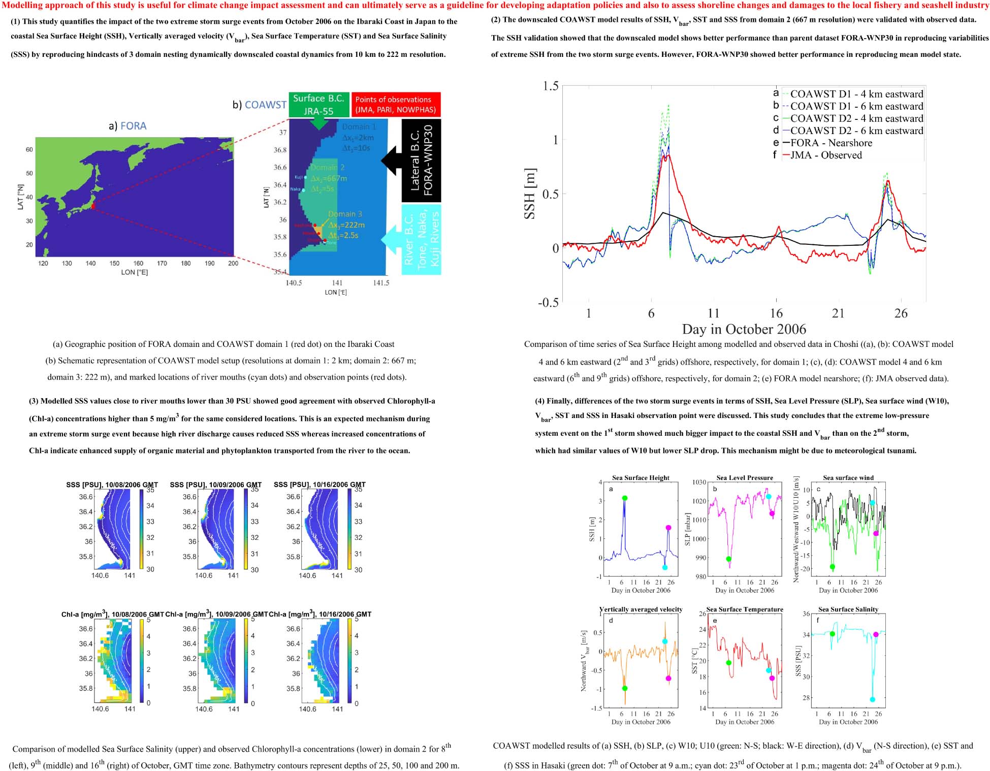
Graphical Abstract. Study domains and model setup (up-left), Sea Surface Height results validation (up-right), Sea Surface Salinity results validation (down-left) and impact of the two storm surge events to the associated coastal dynamics variables (down-right).

Introduction

Storm surge is a coastal phenomenon which has been occurring recently with increasing frequency due to the impact of climate change. Consequently, an increase is projected in the global mean sea level and other oceanic and atmospheric parameters (Intergovernmental Panel on Climate Change (IPCC), 2014). Coastal zones are particularly susceptible to the effects of climate change because of shallow water environment where, as opposed to deeper oceanic waters, a little change in any oceanic parameter [e.g., Sea Surface Height (SSH), vertically averaged velocity (V_bar), Sea Surface Temperature (SST), and Sea Surface Salinity (SSS)]; in any atmospheric parameter, [e.g., Sea Level Pressure (SLP) or surface wind]; or in any fluvial parameter (e.g., river discharge), can cause a much bigger impact on the coastal environment or local fishery and seashell industry. The mutual interplays of all of these coastal parameters are important in reproducing hindcasts of storm surge events. Since coarse resolution scale global climate models cannot precisely reproduce hindcasts of these coastal parameters, the downscaling of coastal dynamics to finer spatiotemporal resolution scales is needed. In the following paragraphs, past related studies with common topic of extreme surge events are discussed according to the spatial scale of relevance for this study: first, similar recent studies outside of Japan are discussed on the example of Typhoon Haiyan in Philippines, then past related studies occurred in Japan are discussed, and afterwards past related studies on the Ibaraki Coast of Japan are discussed. Finally, it is pointed out the literature gap which is missing in all those related studies, which is therefore the objective of this study.

Many recent studies about extreme storm surge events focus, for example, on the extreme super Typhoon Haiyan which struck the Philippines in 2013. Mori et al. (2014) found that the Haiyan storm surge was about 5–6 m high and wind-induced surge and bay oscillation caused extreme surge height. Lagmay et al. (2015) documented the storm surge simulations which were used as basis for the warnings provided to the public 2 days prior to the howler’s landfall. Takayabu et al. (2015) indicated that the worst case scenario of a storm surge in the Gulf of Leyte may be worse by 20% due to the already occurred global warming since 1870. Lee and Kim (2015) parametrized the wave-induced dissipation stress from breaking waves, whitecapping and depth-induced wave breaking. Kim et al. (2015) found that determination of the radius of the Typhoon is important to simulate the Haiyan surge and wave heights inside of the Leyte Gulf. Soria et al. (2016) compared Haiyan storm surge heights with its predecessor from 1897, which had similar heights on the open Pacific Coast but the heights were twice lower than in San Pedro bay. Takagi et al. (2016) evaluated the impact of flood waters caused by the storm surge on evacuation in urban areas, and recommended that evacuation of pedestrians during a storm peak is usually more hazardous than allowing them to stay in their homes. Kumagai et al. (2016) estimated the return periods of storm surge levels to be 240 to 360 years. Tajima et al. (2016) carried numerical experiments to investigate dynamic behavior of storm surge and storm waves on San Pedro bay and found that the bay seiche may be one of the dominant factors that amplify the surge height at the inner part of the bay. Al Mohit et al. (2018) showed that the maximum water level of the storm surge was reduced by up to 20% near the river mouth due to the penetration of piled up water inside the Meghna River if the impact of freshwater inflow was considered in the coastal ocean model, thus, making it important to include rivers when conducting storm surge simulations. Khanal et al. (2019) analyzed near-simultaneous occurrence of high river discharge and storm-surge peak and found that the hazard of their co-occurrence cannot be neglected in a robust risk assessment. Ye et al. (2020) united traditional hydrologic and ocean models in a single modeling platform to show that the baroclinicity was a major driving force in adjustment phase of rebounding water level and the sustained high water-level during the ensuing river flooding for the Hurricane Irene event in 2011. Höffken et al. (2020) emphasized the high importance of uncertainty related to temporal variability of storm surge events on flood characteristics in coastal zones. Tadesse et al. (2020) simulated storm surges at the global scale using data-driven models and showed that mean sea-level pressure is the most important predictor to model daily maximum surge. The most recently, Muis et al. (2020) projected a high resolution global dataset of extreme sea levels, tides and storm surges for the period 1979–2017 as well as future climate projections from 2040 to 2100.

In Japan, there have been many studies of hindcasts, forecasts and future projections of extreme storm surges that are mainly induced by extreme typhoons or low-pressure events. Higaki et al. (2009) developed a numerical storm surge model to provide the basis for warnings to mitigate the effects of such disasters. Kim et al. (2010) showed that wave-induced set-up is important for determining storm surge water levels during Typhoon Anita. Lee et al. (2010) developed a new method for wave–current interaction in terms of momentum transfer due to whitecapping in deep water and depth-induced wave breaking in shallow water for storm surge events in Seto Inland Sea for Typhoons Yancy and Chaba. Kim et al. (2014) found that the characteristic of the after-runner storm surge from Typhoon Songda comes from the Ekman setup which is impacted by the Coriolis force over the Tottori Coasts. Ninomiya et al. (2017) conducted dynamical downscaling to study present and future climate conditions and storm surge simulation for Typhoon Vera. Troselj et al. (2017) found that the impact of freshwater outflow on sea surface salinity during and after Typhoons Roke and Chataan was significant. Mori et al. (2019a) presented the maximum storm surge of 3.29 m at the Osaka Tide Station and analyzed the relation between maximum water level and the resulting damage from Typhoon Jebi of 2018. Mori et al. (2019b) projected that extreme storm surge will be accelerated by global warming with the similar magnitude to sea-level rise in + 4K condition, which represents future climate experiments of 2051–2110 years × 90 members.

On the Ibaraki Coast of Japan, several past studies have focused on the longshore current driving forces and hindcasts of extreme storm surge events. Goda (2006) showed that various current driving forces other than waves are important for generating longshore currents. Nobuoka et al. (2007) specifically analyzed the driving force of storm surge in the October 2006 event and the maximum water level recorded along the coast. They reported that the Ekman transport was the main physical force that generated this high tide level and that unusual time and spatial distribution of winds around the low-pressure system considerably affected the force. Makino and Nobuoka (2016) probabilistically estimated storm surge and showed that it was possible to minimize local variations by regional frequency analysis and to predict average storm surge inundation. Endo et al. (2017) found that the low salinity waters from Tone River sometimes flow into the coastal zone of Kujukuri due to southward current flow and that warm waters sometimes flow toward Kashima-Nada. More recently, Troselj et al. (2018) and Troselj et al. (2019) conducted dynamical downscaling of coastal dynamics emphasizing freshwater impact from three major rivers and seasonal variabilities of SST and SSS, respectively. Furthermore, several past studies focused on shoreline variabilities along the Ibaraki Coast (Takewaka and Galal, 2007, 2015; Suzuki and Kuriyama, 2014; An, 2016; Banno et al., 2016; Takewaka and Wen, 2017), with some of them dealing with impacts due to the October 2006 storms. Galal and Takewaka (2011) conducted erosion analyzes along the Kashima Coast in Ibaraki for the extreme October 2006 storm from the viewpoint of wave energy flux distribution. The M2 tidal constituent dominates on the Ibaraki Coast with the approximate astronomical tidal range from 0.6 m until 1.5 m. Furthermore, Takewaka and Galal (2007) and Galal and Takewaka (2011) showed that the maximum astronomical tidal range were 1.5 and 1.2 m, maximum significant wave heights were 7 and 6 m and maximum wave periods were 14 and 12 s in the considered study domains during the two extreme October 2006 storms, respectively. The stronger of the two extreme storm surge events from October 7 is referred as S1, while the weaker one from October 24 is referred as S2 hereafter.

While the simulation of SSH during extreme storm surge events have been the focus of most of the above-mentioned studies, other oceanic parameters occurring simultaneously with the extreme events (e.g., V_bar, SST, or SSS) have not yet been accurately quantified. Such quantification of parameters on fine resolution spatial and temporal scales is essential for accurate assessment of an extreme storm surge event. Furthermore, the coastal erosion processes on the Ibaraki Coast are numerous and are mostly induced by the coastal current as a result of strong winds, which is why most previous studies focused on shoreline variabilities along the Ibaraki Coast. These studies, however, did not take into consideration accurate hindcasts of coastal ocean currents on fine resolution spatial and temporal scales to enhance the analysis of their results. Reproducing hindcasts of the downscaled fine resolution scale coastal ocean current is important to quantitatively improve analysis of the surge heights and high velocities which can induce shoreline change. Moreover, quantification of variations in water temperature and salinity for extreme storm surge events is important to properly understand and assess the significant impacts on the well-developed local fishery and seashell industry on the Ibaraki Coast, so that improved countermeasures can be implemented in future. Furthermore, the comprehensive results of this study and its modeling approach can also be useful for climate change impact assessment and ultimately serve as guidelines for developing adaptation policies.

The objective of this study is to quantify the impact of the two extreme storm surge events in October 2006 on the Ibaraki Coast in Japan to the coastal SSH, V_bar, SST, and SSS by reproducing hindcasts of downscaled coastal dynamics from coarse resolution (10 km) of global scale to 222 m resolution in local scale. Changes in values of the identified parameters in the downscaled and parent datasets are compared and discussed in this study.

Dynamical Downscaling Methodology

Model Setup

In this study, Coupled-Ocean-Atmosphere-Wave-Sediment-Transport Modeling System (COAWST), as described in Warner et al. (2010), was used for dynamical downscaling computations. COAWST is a terrain-following 3D primitive Euler equation ocean circulation model for curvilinear coordinate with the hydrostatic and Boussinesq approximations. The 1-year COAWST model run, with detailed methodology described in Troselj et al. (2019), started with an initial ocean state condition on January 1, 2006 and ended on December 31, 2006. The analyzed model run between the two studies is the same, but this study provides a more detailed and comprehensive validation of the model parameters by separately validating four coastal dynamics parameters. Furthermore, this current study also analyses time series data of each S1 and S2 with focus on more comprehensively analyzed impact of the storm surge events to multiple coastal dynamics parameters, while the previous study analyzed seasonal and inter-annual variabilities of SSS and SST.

Methods for dynamical downscaling from the ocean reanalysis dataset Four-dimensional Variational Ocean ReAnalysis for the Western North Pacific over 30 years, FORA-WNP30, with 10 km resolution and daily output values (FORA, Usui et al. (2017)) were developed using COAWST model with 2 km resolution and hourly output values. Figure 1A shows the geographic position of FORA domain and COAWST domain 1 on the Ibaraki Coast. The COAWST model used 3 domain nesting with 2 km (domain 1), 667 m (domain 2) and 222 m (domain 3) resolution and 10, 5, and 2.5 s baroclinic time steps, respectively, in the horizontal and 30 sigma layers in the vertical. Although choice of the largest domain for downscaling is arbitrary, the size of domain 1 was determined based on target area for downscaling, water depth and grid coverage in parent domain by FORA. The sensitivity of estimated optimal model spatial resolutions from 2 km, 667 m and to 222 m was checked for SSH and V_bar (not shown in the manuscript). The sensitivity of estimated optimal model temporal resolutions from 10, 5, and 2.5 s was checked in terms of running stability and total duration of the simulation (not shown in the manuscript). When estimating model domains extent, consideration was given so that the offshore boundaries should not be too close to shoreline (< Δx of forcing) but also not so far for downscaling. The finest domain resolution covered Hasaki observation point and was set to 222 m for assessing coastal current in the shallow water environment. The COAWST model does not include astronomical tides directly by itself, but tides can be included from the parent dataset FORA on all four lateral boundaries numerically. This study focus on storm surge height excluding astronomical tide. Figure 1B schematically shows the setup of the COAWST model, extent of the domains and locations of marked river mouth and observation points, which were used for validation.

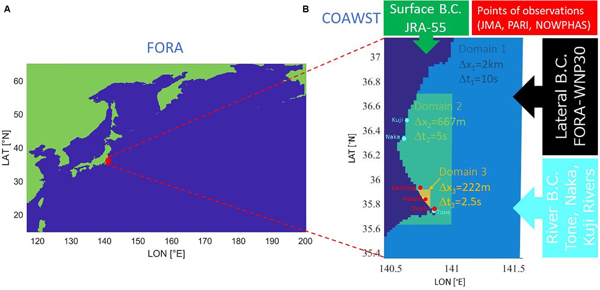
Figure 1. (A) Geographic position of FORA domain and COAWST domain 1 (red dot) on the Ibaraki Coast; (B) Schematic representation of COAWST model setup (resolutions at domain 1: 2 km; domain 2: 667 m; domain 3: 222 m), and marked locations of river mouths (cyan dots) and observation points (red dots).

Lateral boundary conditions of three dimensional velocity, temperature and salinity as well as two dimensional SSH were given by FORA with open boundary conditions Chapman-implicit (free surface, from Chapman, 1985), Flather (2D momentum, from Flather, 1976) and Gradient (3D momentum, mixing turbulent kinetic energy, temperature and salinity). The sea surface initial and boundary conditions were given by the atmospheric reanalysis JRA-55 (Ebita et al., 2011; Kobayashi et al., 2015) with 55 km spatial resolution averaged to the COAWST model domain sizes, and three hourly data resolution averaged to six hourly input data to the COAWST model. The applied atmospheric forcing were wind speed, sea level pressure, air temperature, relative humidity, precipitation, shortwave radiation flux, and cloud fraction. The same methodology for the sea surface initial and boundary conditions was used in FORA.

The bathymetry M7000 Digital Bathymetric Chart obtained by Japan Hydrographic Association (JHA) (2019) submarine topography digital data was used for making grid data. The resolution of the bathymetry input to the model was 10–50 m, depending on the water depth. Observed hourly river water temperature and discharge data were obtained from Japan’s Ministry of Land, Infrastructure, Transport and Tourism (MLIT) (2017). River forcing boundary conditions were used as an assumed constant salinity of 0.5 PSU for Tone, Naka, and Kuji Rivers. As an example of Tone River, the observed river water temperature and discharge data were obtained from the closest observation station to the river mouth which was not affected by tides, and then (for discharge only) multiplied by the ratio between the river mouth’s and the station’s basin areas, with goal to realistically represent freshwater budget flowing into the ocean on the river mouth location, rather than on the upstream observation station location. Hourly river discharge data were obtained from Fukawa station, located 76.47 km upstream from the river mouth and with the station’s basin area of 12,458 km². However, Tone River has total basin area of 15,872 km², so all the obtained discharge data were multiplied by factor 15,872/12,458, as described above. River discharge data were available for the majority of the periods and eventual missing data were obtained by discharge-stage (Q-H) curve relationship. River water temperature data were obtained from Sawara station, located 40.8 km upstream from the river mouth in irregular intervals during daytime, approximately once per month, and data for missing periods were obtained by linear interpolation of two consecutive measurements. The same principal methodology for obtaining river water temperature and discharge data was used for Naka and Kuji Rivers.

Model Validation

The COAWST downscaled results of SSH, V_bar, SST and SSS from domain 2 (667 m resolution) in October 2006 were validated against observed measurements.

Time series of modeled SSH, V_bar, and SST were validated against observed coastal data obtained as filtered values of hourly deviation from astronomic tide from the Japan Meteorological Agency (JMA) (2020) in Choshi (SSH), hourly variations of mean current from The Nationwide Ocean Wave information network for Ports and HArbourS (NOWPHAS) (2019) in Kashima (V_bar) and hourly ocean water temperature from Port and Airport Research Institute (PARI) (2018) in Hasaki (SST). These modeled results were also compared with the parent dataset FORA from September 28 to October 27 in order to highlight the importance of downscaling and the necessity of including river forcing boundary conditions, since river forcing was not considered in FORA.

The modeled results of SSS were validated with observed remote-sensing Version 4.0 of European Space Agency Ocean Color Climate Change Initiative Level 3 mapped Chlorophyll-a concentration (hereafter: Chl-a) data [Sathyendranath et al., 2012; Troselj et al., 2017; European Space Agency Ocean Colour Climate Change Initiative (ESA-OC-CCI), 2019], that comprises globally merged MERIS, Aqua-MODIS, SeaWiFS and VIIRS data with associated per-pixel uncertainty information obtained at 4 km and 1-day resolution. The observed Chl-a data were obtained for October 8, 9 and 16 because for other dates were the data coverage was not sufficient.

Before analysis, model bias correction was applied for SSH and SSS data of COAWST and SSH data of FORA modeled results, with added +0.49 m SSH and +3 PSU to SSS to the entire COAWST dataset as well as +0.33 m SSH to the entire FORA dataset. The SSH bias has occurred since the beginning of simulation due to numerical computational error at the start of modeling (model spin-up) and has remained constant during the simulation. The SSS bias has occurred instantly during extreme rainfall events in the typhoon season when salinity has suddenly been decreased for about 3 PSU over entire modeled domains and has remained low afterward during the simulation.

Results and Discussion

In this section, the validation of SSH, V_bar, SST, and SSS are separately presented. After multiple validation of the modeled results, an analysis was made of the impact of the event to SSH, SLP, Sea Surface northward Wind (W10), V_bar, SST, and SSS in Hasaki point as well as to Tone and Naka River discharges, from September 28 to October 27.

Sea Surface Height

Validations of the COAWST downscaled SSH results from various aspects are presented in this section.

Figure 2A shows peak SSH horizontal distribution from onshore to 6 km eastward offshore at Choshi. The results are shown for COAWST domain 1 and domain 2 for S1 and S2 and compared with surge data observed by JMA at Choshi Tidal Station at location N 35°45′ and E 140°52′. The modeled results in domain 2 show maximum of 1.6 and 0.75 m nearshore for the two considered storms, respectively, which is due to the sudden increase of SSH during the extreme storm surge events in shallow water environments. These results are overestimating observed data because the effect of amplified nearshore SSH increases the modeled results in shallower waters. The exact JMA observation location is located within the Choshi Fishing Port which is semi-enclosed to open ocean and, therefore, the full effect of amplified nearshore SSH is not recorded in the observed data. Furthermore, the modeled results show clear resolution dependence of storm surge height, as maximum SSH in domain 1 are 2.3 and 1.05 m nearshore for the two considered storms, respectively. Therefore, modelled SSH domain 2 results from 4 to 6 km eastward offshore from Choshi are validated with the tide data observed by JMA at Choshi Tidal Station. Figure 2B shows peak SSH horizontal distribution from onshore to 6 km eastward offshore at Hasaki. The results are shown for COAWST domain 1, domain 2 and domain 3 for S1 and S2. Observed SSH data for Hasaki are not available. Maximum nearshore SSH values in Hasaki are up to 3.2 m and 1.6 m for S1 and S2, respectively, which is bigger than in Choshi because Hasaki is located at a longshore uniform section, while Choshi is at the tip point of a cape where the direction of coastline changes sharply. Furthermore, the results in Hasaki do not show noticeable resolution dependence of storm surge height which might be due to smaller variabilities of magnitudes and directions of ocean currents in the Hasaki longshore uniform section than in the Choshi tip point of a cape.

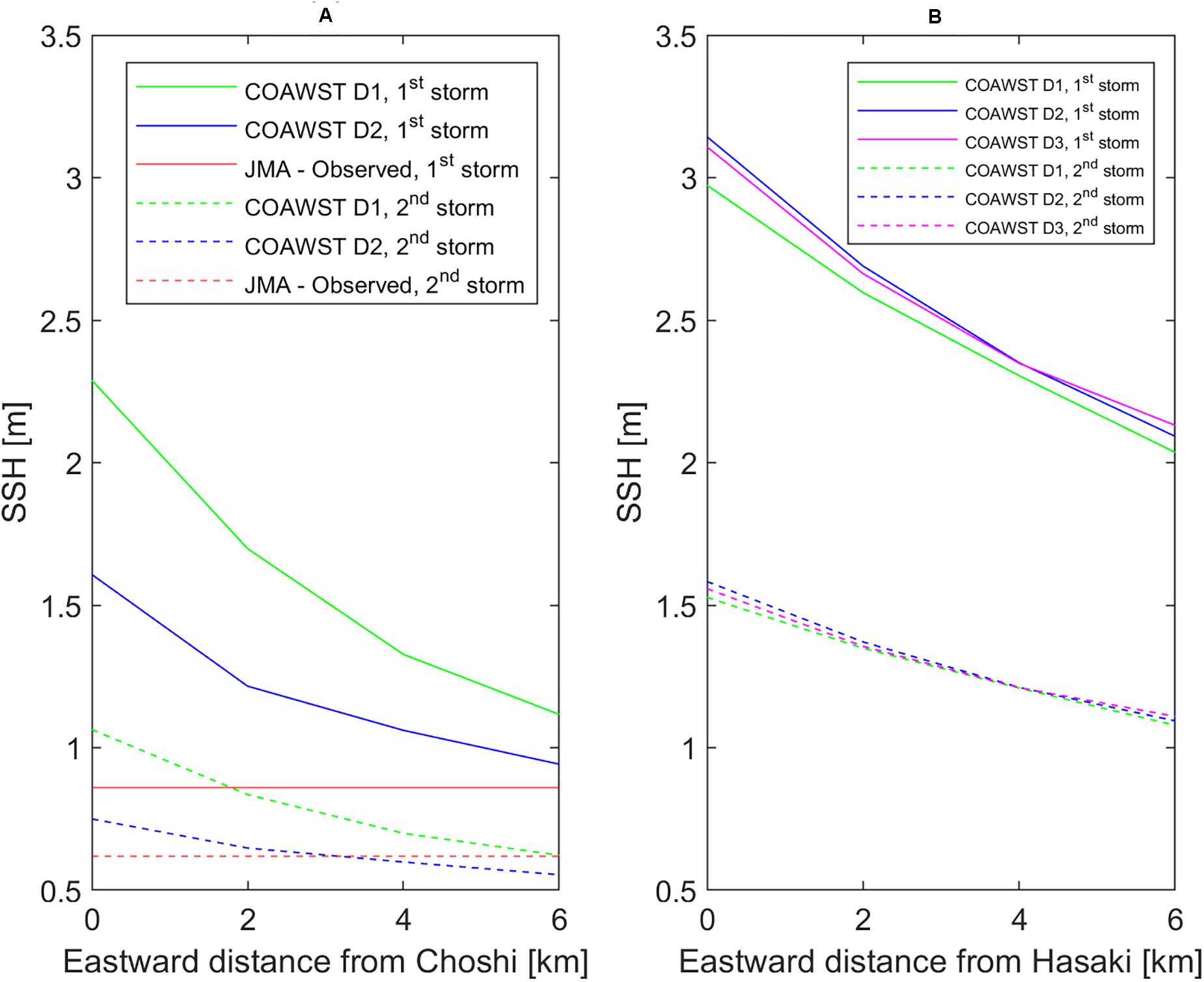
Figure 2. Peak Sea Surface Height horizontal distribution from onshore to 6 km eastward offshore at (A) Choshi and (B) Hasaki for COAWST domain 1 (green), domain 2 (blue) and domain 3 (magenta, only in Hasaki) for S1 (full line) and S2 (dashed line) compared with surge data observed by JMA at Choshi Tidal Station (red, only in Choshi).

Figure 3 shows comparison of time series of SSH among (a) FORA results nearshore and the modeled results, (b) 4 km and (c) 6 km eastward offshore from Choshi for domain 1, and (d) 4 km and (e) 6 km for domain 2, and (f) tide data observed by JMA at Choshi Tidal Station. Results at various distances from the shoreline are shown because it was observed that sensitivity of location from offshore to onshore in terms of SSH is significant, being inversely proportional to water depth. The modeled results show good agreement with peaks of observed data from both S1 and S2 (0.8 and 0.6 m, respectively) at a few grids locations, 4–6 km (2nd and 3rd grids in domain 1, 6th and 9th grids in domain 2) eastward offshore from Choshi, while peaks of FORA for the same events are not well reproduced (about 0.25 and 0.2 m, respectively). As the wind-induced surge monotonically increases from offshore to onshore and spatial scale of storm surge is small, spatial resolution is sensitive to simulate maximum storm surge heights along the coast. Besides the spatial resolution, another factor causing the huge difference between COAWST and FORA results is temporal output resolution, which is hourly in COAWST but daily in FORA. Therefore, physical processes which are mainly occurring on hourly time scales such as the considered S1 and S2 cannot be realistically reproduced by FORA and because of that finer spatiotemporal modeling scales are needed for their reproducibility. Additionally, the JMA sea level observation data are filtered values but COAWST modeled output data are just one data output per every hour and FORA modeled data are also just one data output but per every day. Therefore, we did not compare the same data obtaining processes which additionally reduced accuracy of the validation process.

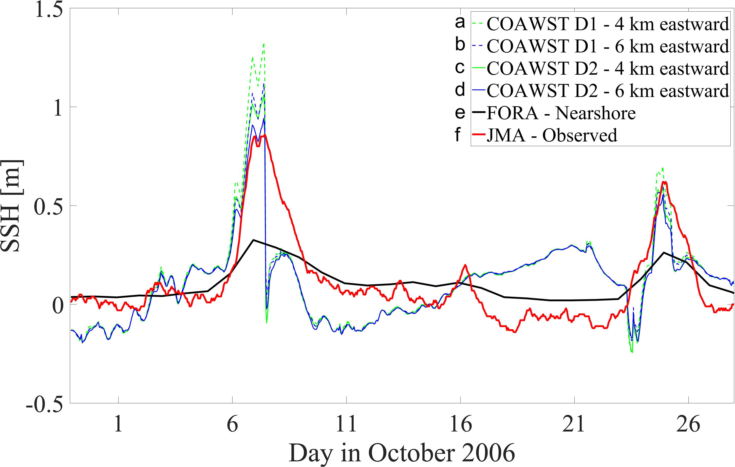
Figure 3. Comparison of time series of Sea Surface Height among modeled and observed data in Choshi [(a,b): COAWST model 4 and 6 km eastward (2nd and 3rd grids) offshore, respectively, for domain 1; (c,d): COAWST model 4 and 6 km eastward (6th and 9th grids) offshore, respectively, for domain 2; (e) FORA model nearshore; (f): JMA observed data].

Table 1 shows correlation coefficient, RMSE and bias of above-mentioned three records from modeled runs (FORA – nearshore, COAWST domain 2 – 4 km and 6 km offshore) for the total analyzed period, S1 on October 7 and S2 on October 24. In Table 1, the modeled results from 4 to 6 km offshore show the best fit with observed data (correlation coefficient 0.54 for total period, 0.55 for S1 and 0.71 for S2, respectively, for 4 km offshore; and 0.52 for total period, 0.58 for the S1 and 0.70 for the S2, respectively, for 6 km offshore). As such, these distances should be used for the best validation of the modeled results, whereas in shallower waters, the effect of amplified nearshore SSH increases the modeled results. FORA results nearshore have higher correlation coefficient of 0.81 for total period but lower correlation coefficients than COAWST of 0.68 for the S1 and 0.48 for the S2, respectively. The correlation coefficient for the S1 is comparable to that of COAWST and FORA, but this is because COAWST underestimates observed data after the peak of S1. However, COAWST results up to the maximal SSH for the S1 is much closer to observed data than FORA. Furthermore, COAWST RMSE is higher than FORA for the total period but lower for S1 and S2. Therefore, the model shows better performance than FORA in reproducing variabilities of ocean state such as the two events’ extreme SSH, while FORA shows better performance in reproducing mean state of the model. The most important feature of downscaling is that it is used for reproducibility of extreme coastal variabilities of the ocean rather than its mean values, because the parent dataset with coarser resolution is already good enough to accurately reproduce its mean values. Bias in COAWST results is smaller by about 13–16 cm than in FORA for S1; and by about 2–3 cm for S2 because FORA does not reproduce hindcasts of S1’s and S2’s peaks well. SSH validation showed that the downscaled model shows better performance than FORA in reproducing peaks and variabilities of extreme SSH from the two events, while FORA shows better performance in reproducing mean state of the model.

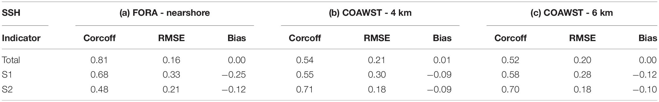
Table 1. Correlation coefficient, RMSE and bias of (a) FORA nearshore and COAWST (domain 2) modeled runs at (b) 4 and (c) 6 km eastward offshore from Choshi for the total analyzed period, S1 and S2.

Finally, we discuss spatiotemporal variation of SSH alongside the Ibaraki Coast. Figure 4 compares time series of modeled SSH from COAWST domains 1 and 2 and FORA on four locations alongside the Ibaraki Coast. The results suggest that magnitude of the SSH was increased from south to north reaching up to 3.8 m for S1 and 2.3 m for S2, respectively. These modeled values of S1 SSH are in range of the most extreme storm surges that have been recorded on the Ibaraki Coast. However, these extreme SSH values for S1 and S2 are not well reproduced in FORA alongside the entire Ibaraki Coast. Figure 4 additionally suggest that differences between domain 1 and domain 2 are minor alongside the Ibaraki Coast but are significant on to most southern point Choshi which was used for the SSH validation. In Choshi, domain 2 SSH results greatly underestimate domain 1 SSH results. These findings suggest that nesting approach is important to reproduce SSH along open coasts.

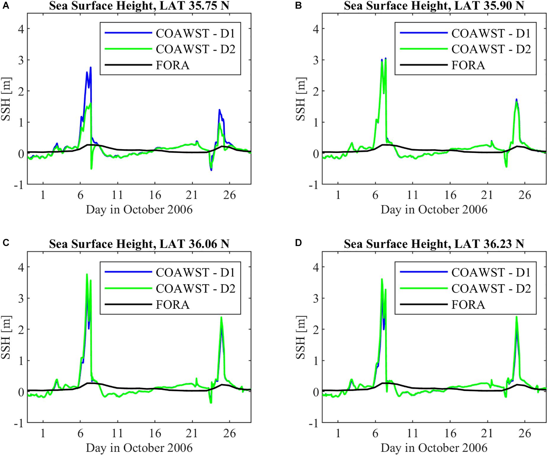
Figure 4. Comparison of time series of modeled Sea Surface Height (blue – COAWST domain 1, green – COAWST domain 2, black – FORA) alongside the Ibaraki Coast on four locations corresponding to LON (A) 35.75 N, (B) 35.90 N, (C) 36.06 N, (D) 36.23 N.

Vertically Averaged Velocity

The validation of the COAWST downscaled V_bar results is presented in this section. Figure 5 shows comparison of time series of V_bar (North-South direction) among the modeled results, FORA results and NOWPHAS observed velocity data in Kashima at location N 35°53′55″ and E 140°45′14″ at depth 24 m by Ultra Sonic Wavemeter (USW). The observed data has no coverage during S1 at October 7 because the USW velocimeter failed to collect data.

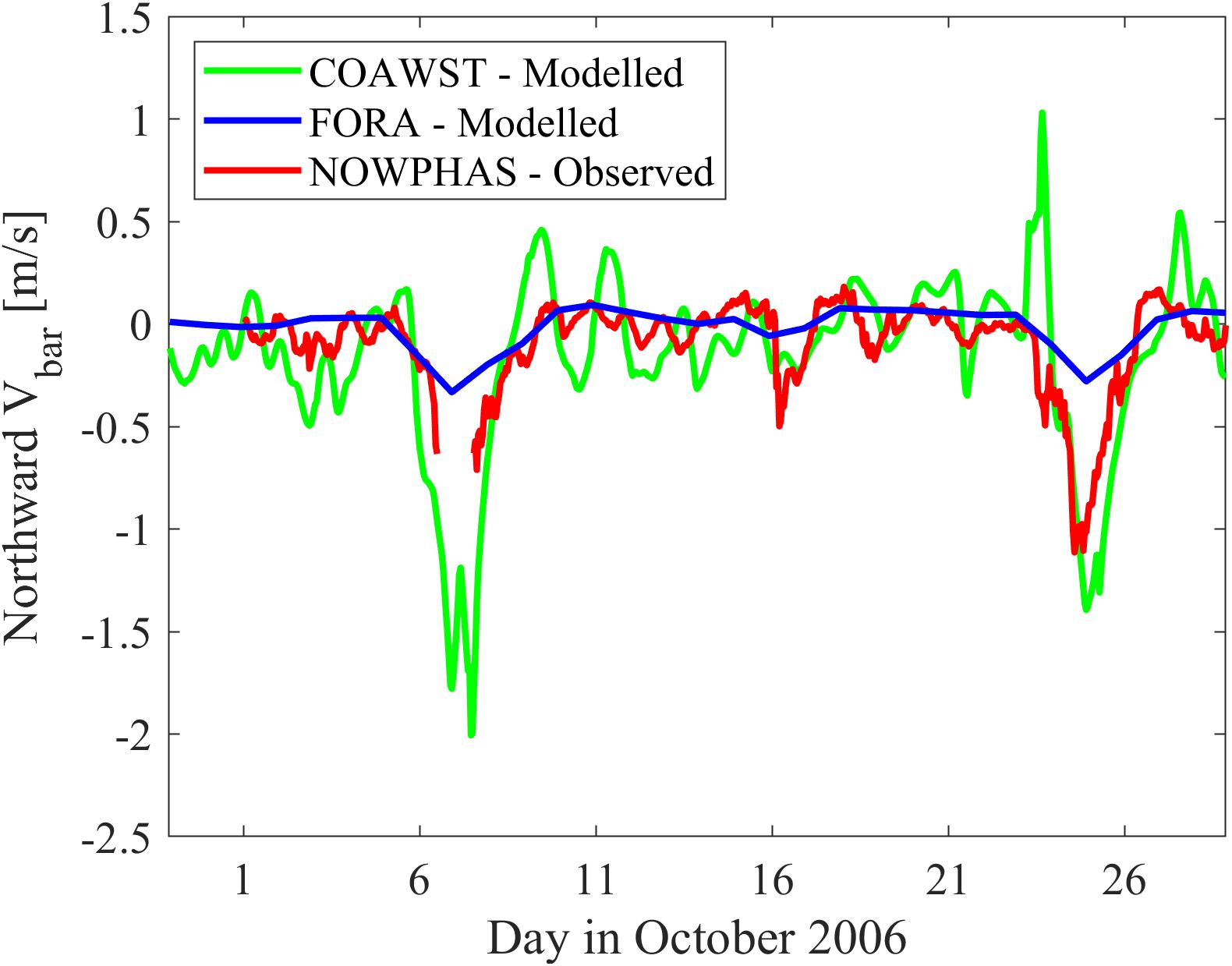
Figure 5. Comparison of time series of vertically averaged velocity (North–South direction) among modeled and observed data in Kashima (green: COAWST model, blue: FORA model, red: NOWPHAS observed data).

The modeled results have correlation coefficient 0.68, RMSE 0.27 and bias −0.03, while FORA has values of 0.63, 0.19, and 0.07, respectively, for total time period when there was available observed data. For the S2, the modeled results show a correlation coefficient 0.68, RMSE 0.44, and bias −0.02, while FORA has values of 0.28, 0.43, and 0.27, respectively. The modeled results show good agreement with the peak of the S2 reproducing hindcasts of extreme velocity of about 1.4 m/s southwards, while FORA hindcasts peak for the same event are not well reproduced, not even exceeding 0.3 m/s. For S1, the modeled results were reaching peak of up to 2 m/s while FORA results peak did not exceed 0.4 m/s. V_bar validation showed similar hindcasts of mean state of the model between COAWST and FORA for total time period, but much better hindcasts of strong southward V_bar for energetic periods by using COAWST.

Sea Surface Temperature

The validation of the COAWST downscaled SST results is presented in this section. Figure 6 shows comparison of time series of SST among the modeled results, FORA results and PARI observed ocean water temperature data in Hasaki located 2–3 m below sea level at location N 35°50′27″ and E 140°45′42″. The observed data has no coverage during both extreme events but show good agreement with the modeled results in other periods, while FORA results slightly overestimate them.

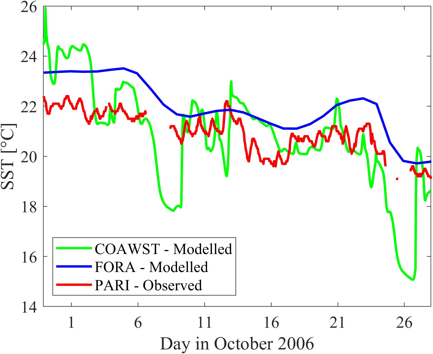
Figure 6. Comparison of time series of Sea Surface Temperature among modeled and observed data in Hasaki (green: COAWST model, blue: FORA model, red: PARI observed data).

The modeled results have correlation coefficient 0.67, RMSE 1.43, and bias 0.19, while FORA has their values at 0.77, 1.30, and 1.14, respectively, for total time period when there was available observed data. This shows that in terms of SST, both the model and FORA show similar hindcasts for normal conditions but the quality of the hindcasts for S1 and S2 is still uncertain due to missing observation data. The modeled results show a decrease in SST of about 4°C during S1 and S2 on October 7 and 24 while FORA shows a smaller decrease of about 2°C for both events. SST validation showed similar hindcasts in both the model and FORA at normal conditions but the quality of the hindcasts for S1 and S2 is still uncertain due to missing observation data. Therefore, it is noted that accurate validation of modeled SST results for S1 and S2 could not be fully conducted.

Sea Surface Salinity

The validation of the COAWST downscaled SSS results is presented in this section. Figure 7 shows the comparison of the modeled SSS results (upper) and ESA-OC-CCI Version 4.0 observed remote-sensing Chl-a concentration data (lower) in domain 2 for October 8 (left), 9 (middle), and 16 (right) GMT time zone, respectively. Only the Figure 7 is shown in GMT time zone, which is +9 h compared to JST time zone used elsewhere in this study, because the observed ESA-OC-CCI data are provided using daily values in the GMT time zone. These three days are used for validation because there are no available observed data on other days due to extensive cloud coverage in the targeted domain. FORA did not include river forcing, so no comparison of SSS results was made between the two models. Modeled SSS values nearshore close to river mouths are below 30 PSU and this shows good agreement with observed Chl-a concentrations higher than 5 mg/m³ for the same locations. This is an expected mechanism during an extreme storm surge event because high river discharge causes reduced SSS whereas increased concentrations of Chl-a indicate enhanced supply of organic material and phytoplankton transported from the river to the ocean. Therefore, there was no expectation for a strong correlation between SSS and Chl-a concentrations in the offshore zone, where freshwater from the river plume could not reach. SSS validation showed that impact of freshwater discharge to lowering SSS and increasing Chl-a concentration values nearshore was greatest just after the extreme storm surge event but diminishes afterward due to lower supply of freshwater, organic material and phytoplankton from rivers.

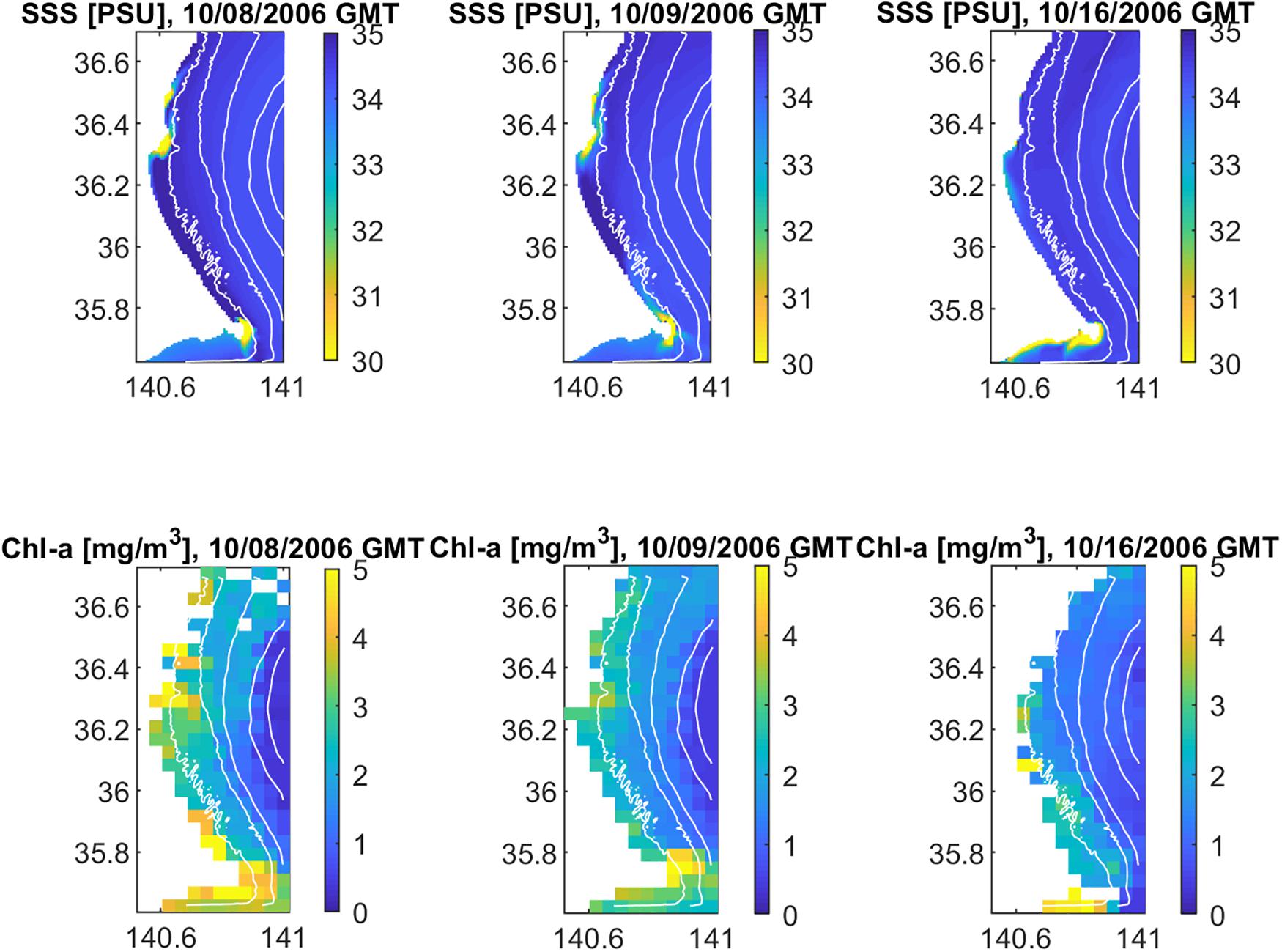
Figure 7. Comparison of modeled Sea Surface Salinity (upper) and observed Chlorophyll-a concentrations (lower) in domain 2 for October 8 (left), 9 (middle), and 16 (right), GMT time zone. Bathymetry contours represent depths of 25, 50, 100, and 200 m.

Furthermore, an evaluation of the impact of freshwater discharge from rivers to SST and SSS values was made. Figure 8 shows observed time series of Tone and Naka River mouth discharge from September 28 to October 27. Kuji River was excluded from this analysis because of its smaller discharge and its location further northward from the considered coastal zone. The peaks of both river discharges occurred during S1 and S2 were reaching 3,200 and 2,000 m³/s for Tone and 1,200 and 800 m³/s for Naka River, respectively. For the considered study domains, these amounts of freshwater discharges are not significant during extreme events when considering hydrological flood disasters, but are large enough to produce significant impact to decreasing SSS and increasing Chl-a concentrations nearshore at aftermaths of extreme storm surge events. By combining Figures 6, 8, it can be concluded that the freshwater impact to SST is minor because river water temperature has similar range of values to ocean water temperatures. By combining Figures 7, 8, on the other hand, it can be concluded that the impact of freshwater discharge to decreasing SSS and increasing Chl-a concentrations nearshore was highest just after S1, on October 8, but decreased on October 9 and further decreased on October 16. It was because freshwater from the river plume changed its location from near river mouths to the southern part of Choshi aftermaths the extreme storm surge event due to influence from southwards coastal currents. It can be concluded that the freshwater impact to SST is negligible but it can have significant impact to reducing SSS, as was likewise concluded in Troselj et al. (2018).

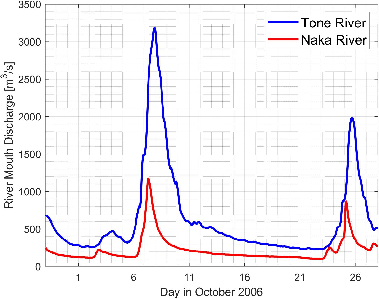
Figure 8. Observed time series of Tone and Naka River mouth discharge from September 28 to October 27 (blue: Tone River, red: Naka River).

Impact of the Storm Surge Events

The impact of the storm surge events in terms of SSH, depth averaged velocity (Overbar{UV}), SST and SSS in domain 2 is discussed in this section.

Figure 9 shows the modeled SSH and Overbar{UV} for October 7 at 9 am, October 23 at 1 pm and October 24 at 9 pm. These particular moments represent three peaks of SSH variation (extreme S1 and S2 on October 7 and 24, and sudden drop of SSH on October 23 with negative SSH peak, when the modeled results show the counter–current flow to the northward direction preceding the following S2). Figure 9A shows that magnitude of SSH for October 7 event exceeded 3 m in the coastal zone of Ibaraki with higher values at the northern part. A similar occurrence mechanism but with lower SSH magnitudes of up to 2.2 m was found for October 24 event (Figure 9C). On the October 23, values lower than zero mean sea level were distributed uniformly across the whole domain with negative peaks nearshore (Figure 9B). Figures 9D,F show that magnitude of Overbar{UV} for October 7 and 24 had similar occurrence mechanism, and both exceeded values of 1 m/s in southward direction from northern part of Choshi toward its coastal zone, with slightly lower values at nearshore. On October 23, the northward velocity approached its maximum of about 0.8 m/s near Choshi and gradually decreased toward the north (Figure 9E). The impact of the extreme storm surge events S1 and S2 was significant especially in terms of SSH and Overbar{UV}, which is important in assessment of erosion analyses and shoreline variabilities along the Ibaraki Coast.

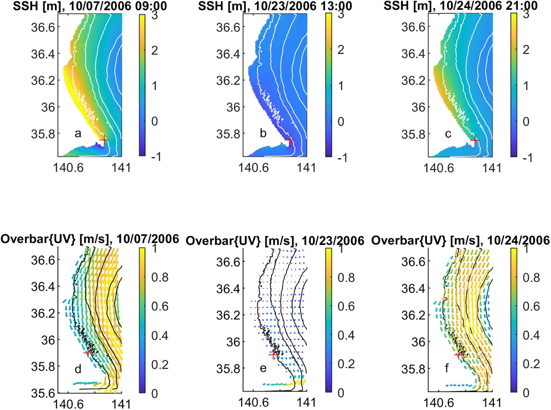
Figure 9. Sea Surface Height (upper) and depth averaged velocity (lower) for October 7 at 9 am (left), October 23 at 1 pm (middle) and of October 24 at 9 pm (right). Bathymetry contours represent depths of 25, 50, 100, and 200 m. Red cross indicates the location of the corresponding observed data.

Similarly, Figure 10 shows the same modeled outputs as Figure 9 but for SST and SSS. There was a dominant impact of strong southward current on October 7 and 24 to coastal transport of colder northern waters of about 16–18°C (Figure 10A), while warmer waters of more than 22°C were trapped on the offshore zone by the strong southward Overbar{UV}. On October 24 (Figure 10C), an SST pattern was observed similar to October 7 but with about 2°C lower average values due to later seasonal period. On October 23 (Figure 10B), the ocean water was warmer by about 1°C than on the October 24 especially in the coastal zone due to the impact of northward currents which transported warmer waters from Kuroshio. There was also an interesting mechanism of SSS coastal transport, which shows that SSS values between 34 and 35 PSU were transported by the southward current on October 7 (Figure 10D, south from LON 35.75), but on October 24, there was a coastal backflow of reduced SSS near Tone River mouth (Figure 10F, around LON 35.75) that had been previously transported alongshore with northward current as a freshwater lens on October 23 (Figure 10E, from LON 35.75 to 35.95). Therefore, the impact of S1 and S2 in terms of SST and SSS might be considerable in possibly causing non-negligible damage to the well-developed local fishery and seashell industry on the Ibaraki Coast.

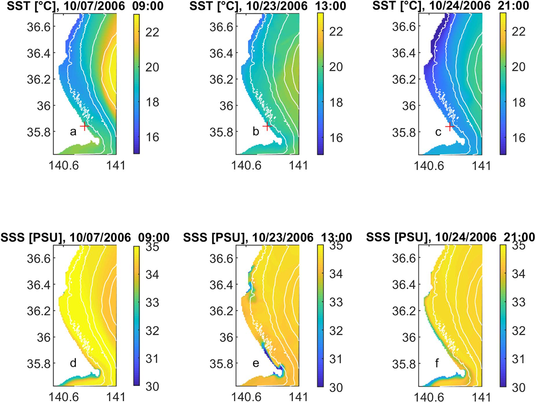
Figure 10. Sea Surface Temperature (upper) and Sea Surface Salinity (lower) for October 7 at 9 am (left), October 23 at 1 pm (middle) and October 24 at 9 pm (right). Bathymetry contours represent depths of 25, 50, 100, and 200 m. Red cross indicates the location of the corresponding observed data.

Finally, differences of S1 and S2 are discussed in terms of the COAWST downscaled results of SSH, SLP, W10, V_bar, SST, and SSS in Hasaki on the same location where SST was validated. Figure 11 shows the results with significantly marked occurrence times at the above-mentioned three extreme SSH events. The SLP (Figure 11B) and W10 results (Figure 11C – green line) show that on October 7, there were both extreme SLP (down to 985 mbar) and strong southward surface wind (up to 20 m/s) occurring simultaneously. However, on October 24, only the southward surface wind (up to 20 m/s) was extreme and its peak was just after the peak of SSH while SLP was in higher range of about 1,010 mbar. Simultaneously, the Sea Surface westward Wind (U10) results (Figure 11C – black line) showed interesting mechanisms during S1 and S2. Peak U10 of up to 13 m/s occurred just after W10 peak of S1 in eastward direction. However, peak U10 of up to 11 m/s occurred just before W10 peak of S2 in westward direction. Additionally, on October 23, SLP was about 1,025 mbar and northward surface wind was about 5 m/s, which generated the reduced SSH with northward alongshore current. These magnitudes and directions of extreme coastal southward surface wind correspond well with the findings from Nobuoka et al. (2007). Therefore, the results under this study might support their conclusion that Ekman transport was the main physical force that generated the high tide level on October 7 and possibly also on October 24.

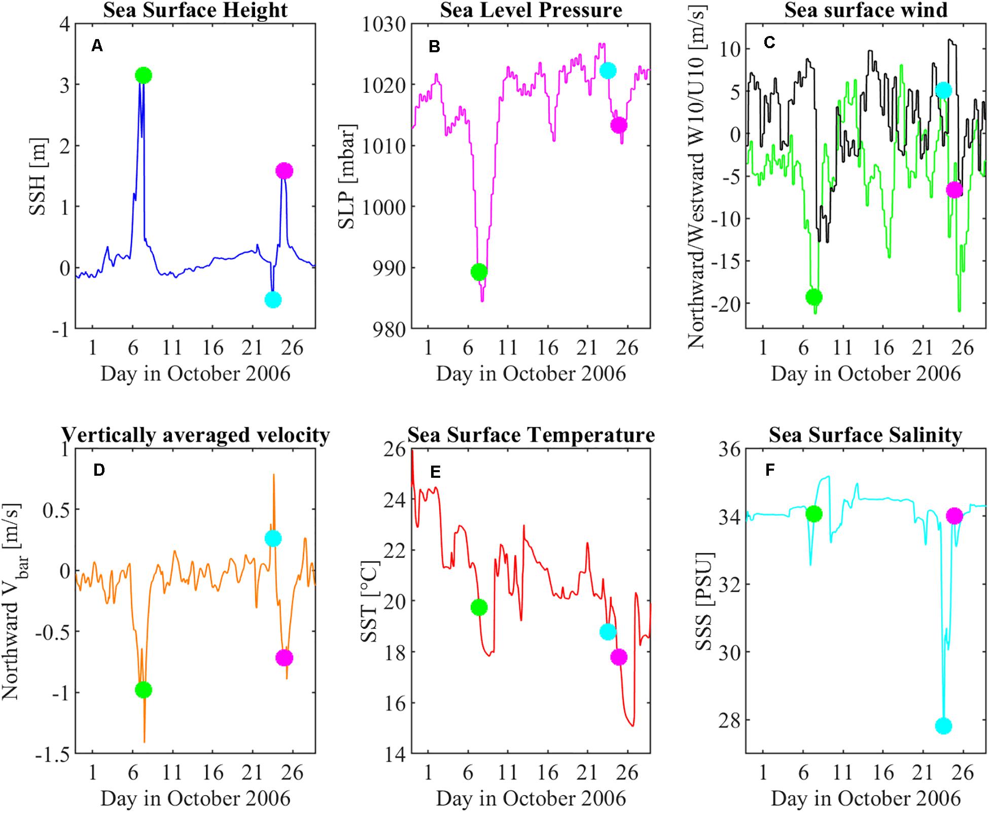
Figure 11. COAWST modeled results of (A) Sea Surface Height, (B) Sea Level Pressure, (C) Sea surface wind (green: North–South direction; black: West–East direction), (D) Vertically averaged velocity (North–South direction), (E) Sea Surface Temperature, and (F) Sea Surface Salinity in Hasaki (green dot: October 7 at 9 am; cyan dot: October 23 at 1 pm; magenta dot: October 24 at 9 pm).

The SSH results (Figure 11A) show that Hasaki was more exposed to extreme storm surge levels than Choshi Tidal Station, because peaks of the SSH in Hasaki reached up to 3 m on October 7 and about 1.8 m on October 24; while in Choshi, they reached up to 1.6 m on October 7 and about 1 m on October 24. On October 23, there were values of about −0.5 m occurring instantly. The V_bar results (Figure 11D) were up to 1.5 and 1 m/s southwards on October the 7 and 24, respectively, and about 0.8 m/s northwards on October 23, which correlates well with the dynamics of coastal SSH occurrence and with coastal transport of SST and SSS. The SST results (Figure 11E) show delayed response to the extreme events. There was an initial decrease of about 2°C occurring about 1 day before the peak of SSH, and further decrease of about 2°C occurring 2 days after the peak of SSH on both October 7 and 24. On October 23, there was no significant change in SST. The SSS results (Figure 11F) show an increase of up to 35 PSU after October 7 event, a decrease up to 28 PSU during the peak northward current on October 23 due to alongshore transport of freshwater lens from Tone River and reverting back to about 34 PSU on October 24 due to coastal backflow of reduced SSS near Tone River mouth.

The extreme low-pressure system event of the S1 showed much bigger impact to the coastal SSH and V_bar than on the S2, which had similar peak values of W10 but a lower SLP drop, while the impact to the coastal SST and SSS was similar. This indicates that the SLP drop itself has an important role in assessing extreme SSH levels, in addition to W10 which directly influences V_bar values. This mechanism of increasing SSH levels might be due to meteorological tsunami, which also occurs when rapid changes in SLP cause the displacement of a body of water as manifested by the rapid increase in SSH levels. However, additional analyses which are not in scope of this study should be conducted to further evaluate this indication.

Conclusion

In this study, dynamical downscaling with reproduced hindcasts of coastal dynamics on the Ibaraki Coast was conducted using COAWST model including SSH, V_bar, SST, and SSS. Particularly highlighted was the importance of downscaling to hindcasts of the two extreme storm surge events in October 2006 on the Ibaraki Coast. The impact of the events to associated values of coastal parameters in the downscaled and the parent datasets was also considered.

Validation of COAWST downscaled results of SSH, V_bar, SST, and SSS from domain 2 (667 m resolution) in October 2006 was made with observed data and a comparison was conducted with FORA to highlight the importance of downscaling. SSH validation showed that the downscaled model shows better performance than FORA in reproducing hindcasts of extreme values of SSH from the two events. As the downscaling model is focused on accurate reproducibility of the coastal variabilities, then its results sometimes differ from mean values due to hourly variabilities in the surface forcing data as well as their uncertainty. However, the downscaling model can be accurately used for objectives that it is designed for, which are reproducibility of hourly extreme variability values of the coastal dynamics parameters. V_bar validation showed better hindcasts of strong southward V_bar for S2, while observed data for October 7 are missing. SST validation showed similar hindcasts in both the model and FORA for normal conditions although the quality of the hindcasts for S1 and S2 is still uncertain due to missing observation data. However, the estimated 2°C bigger decrease of SST in this study’s model than in FORA indicates that the model can better reproduce hindcasts of the local southward alongshore transport of SST during extreme events. SSS validation showed that impact of freshwater discharge to decreased SSS lower than 30 PSU and increased Chl-a concentrations bigger than 5 mg/m³ nearshore is the greatest just after S1, on October 8, but decreases afterward. These validations with existing observed data satisfactorily showed goodness of fit for the two events for all considered coastal dynamics parameters.

Turning to the modeled SSH, Overbar{UV}, SST and SSS results in domain 2, magnitude of SSH was about 3 and 2.2 m for the two events, respectively, with larger values at northern part of the Ibaraki Coast. Magnitude of Overbar{UV} for the two events had similar occurrence mechanism and both exceeded values of 1 m/s in southward direction in position from northwards of Choshi toward its coastal zone. The dominant impact of strong southward current to coastal SST transport of colder northern waters of about 16–18°C occurred during both extreme events. SSS transport of the freshwater lens from rivers was dependent on directions of extreme currents before and during the two events. It was shown that the impact of S1 and S2 was significant particularly in terms of SSH and Overbar{UV}, which is important for assessment of erosion analyses and shoreline variabilities along the Ibaraki Coast. The impact of S1 and S2 in terms of SST and SSS might be considerable for the local fishery and seashell industry on the Ibaraki Coast.

Moreover, the impact of the two events in Hasaki was quantified. It was found that that the main difference in atmospheric forcing between the two events was in SLP, with peak down to 985 mbar on October 7 but about 1,010 mbar on October 24, while strong W10 occurred in both cases with peaks up to 20 m/s. The SSH results show that Hasaki (3 and 1.6 m, respectively) was more exposed to extreme storm surge levels than Choshi (1.8 and 1 m, respectively) during both S1 and S2. The V_bar results show up to 1.5 and 1 m/s southward currents for the two events. The SST results show 2 days delayed response to the extreme event of up to −4°C during both events. The SSS results show a decrease of down to 28 PSU during the peak northward current on October 23, due to alongshore transport of freshwater lens from Tone River. This study concludes that the extreme low-pressure system event on October 7 had much bigger impact to the coastal SSH and V_bar than that on October 24, which had similar peak values of W10 but a lower SLP drop, whereas the impact to the coastal SST and SSS was similar.

Limitations of the modeled results are the COAWST modeled SSH (−0.49 m) and SSS (−3 PSU) biases, which did not significantly affect results after applying bias corrections. However, it is important to account for the SSH and SSS biases in future studies by using improved methodology in order to reduce them, when possible. Another considerable limitation is that the validation of SSH results was conducted by comparing daily modeled outputs from FORA with hourly modeled outputs from COAWST and validating them with filtered JMA hourly observed values. Therefore, different temporal resolutions of validated results and different way of the data obtaining processes decreased reliability of intended considering the impact of increasing spatial resolution because the temporal resolution effect is also important in consideration of explaining the observed differences. Additional limitation to note is that the COAWST downscaled results have too coarse resolution to sufficiently represent physical processes within the Choshi Fishing Port, which is semi-enclosed to open ocean. Therefore we believe that the physical processes within the Port are in range of less than 100 m of spatial resolution whereas in this study the same location was downscaled of down to 667 m. Because of this limitation, we used indirect validation of modeled SSH results on locations from 4 to 6 km offshore versus observed data in the Port.

In future studies, an assessment of erosion analyses and shoreline variabilities along the Ibaraki Coast, as well as future projection analysis of the coastal dynamics using the COAWST model, which was validated in this study, will be conducted. The modeling approach used in this study, with differently applied lateral and surface boundary forcing conditions, can be useful for similar modeling of climate change impact assessment and can ultimately serve as guidelines for developing adaptation policies.

Data Availability Statement

The raw data supporting the conclusions of this article will be made available by the authors, upon a reasonable request to the corresponding author.

Author Contributions

JT compiled, pre-processed and ran the COAWST model, conducted post-processing data analysis as well as wrote and edited the whole manuscript. JN assisted to compile, pre-process and run the COAWST model. ST obtained NOWPHAS mean current data and assisted in post-processing data analysis. NM coordinated the work among all co-authors by conceptually leading the study, provided the working environment for JT and assisted to compile, pre-process and run the COAWST model. All authors reviewed, discussed and suggested revisions for the submitted and revised versions of the manuscript.

Funding

The study was conducted under the Social Implementation Program on Climate Change Adaptation Technology (SI-CAT), Integrated Research Program for Advancing Climate Models (TOUGOU) Grant Number JPMXD0717935498 and Japan Society for the Promotion of Science (JSPS) Grants-in-Aid for Scientific Research (KAKENHI), all supported by the Ministry of Education, Culture, Sports, Science and Technology, Japan (MEXT).

Conflict of Interest

The authors declare that the research was conducted in the absence of any commercial or financial relationships that could be construed as a potential conflict of interest.

Acknowledgments

The authors are grateful to Yoichi Ishikawa and Shiro Nishikawa from Japan Agency for Marine-Earth Science and Technology for providing modeled data from the parent dataset FORA-WNP30 and to Masayuki Banno from Port and Airport Research Institute for providing observed water temperature data in Hasaki. We appreciate NOWPHAS wave data provided by Ministry of Land, Infrastructure, Transport and Tourism, Japan. Finally, we thank to the Associate Editor Goneri Le Cozannet and two Reviewers, Pushpa Dissanayake and Begoña Pérez-Gómez, for their useful comments which greatly improved quality of the manuscript.

References

Al Mohit, M. A., Yamashiro, M., Hashimoto, N., Mia, M. B., Ide, Y., and Kodama, M. (2018). Impact assessment of a major River basin in Bangladesh on storm surge simulation. J. Mar. Sci. Eng. 6:99. doi: 10.3390/jmse6030099
An, S. (2016). A Study on the morphological characteristics around artificial headlands in Kashima coast. Japan. J. Coast. Res. 32, 508–518. doi: 10.2112/jcoastres-d-15-00122.1
Banno, M., Kuriyama, Y., and Takewaka, S. (2016). Large scale shoreline advancement on the Hasaki coast in the past 50 years. J. Japan Soc. Civ. Eng. Ser. B2 (Coast. Eng.) 72, 661–666. doi: 10.2208/kaigan.72.i_661
Chapman, D. C. (1985). Numerical treatment of cross-shelf open boundaries in a Barotropic coastal ocean model. J. Phys. Oceanogr. 15, 1060–1075.
Ebita, A., Kobayashi, S., Ota, Y., Moriya, M., Kumabe, R., Onogi, K., et al. (2011). The Japanese 55-year reanalysis ‘JRA-55’: an interim report. Sci. Online Lett. Atmos. 7, 149–152. doi: 10.2151/sola.2011-038
Endo, J., Sugimatsu, K., Yagi, H., Udagawa, T., Oguchi, S., Ohmura, Y., et al. (2017). Study on numerical ocean model in coastal regions of Kashima-Nada and Kujukuri. J. Japan Soc. Civ. Eng. Ser. B2 (Coast. Eng.) 73, 1171–1176. doi: 10.2208/kaigan.73.i_1171
European Space Agency Ocean Colour Climate Change Initiative (ESA-OC-CCI) (2019). Available online at: https://esa-oceancolour-cci.org/ (accessed August 23, 2019).
Flather, R. A. (1976). A tidal model of the North-West European continental shelf. Mém. Soc. R. Sci. Liège 6, 141–164.
Galal, E. M., and Takewaka, S. (2011). The influence of alongshore and cross-shore wave energy flux on large- and small-scale coastal erosion patterns. Earth Surf. Process. Landf. 36, 953–966. doi: 10.1002/esp.2125
Goda, Y. (2006). Examination of the influence of several factors on longshore current computation with random waves. Coast. Eng. 53, 157–170. doi: 10.1016/j.coastaleng.2005.10.006
Higaki, M., Hayashibara, H., and Nozaki, F. (2009). Outline of the Storm Surge Prediction Model at the Japan Meteorological Agency. Tokyo: Japan Meteorolological Agency.
Höffken, J., Vafeidis, A. T., MacPherson, L. R., and Dangendorf, S. (2020). Effects of the temporal variability of storm surges on coastal flooding. Front. Mar. Sci. 7:98. doi: 10.3389/fmars.2020.00098
Intergovernmental Panel on Climate Change (IPCC) (2014). Climate Change 2014: Synthesis Report. Contribution of Working Groups I, II and III to the Fifth Assessment Report of the Intergovernmental Panel on Climate Change. Geneva: IPCC.
Japan Hydrographic Association (JHA) (2019). Available online at: https://www.jha.or.jp/en/jha (accessed June 26, 2019).
Japan Meteorological Agency (JMA) (2020). Available online at: https://www.data.jma.go.jp/gmd/kaiyou/db/tide/genbo/genbo.php?stn=CS (accessed March 19, 2020).
Khanal, S., Ridder, N., de Vries, H., Terink, W., and van den Hurk, B. (2019). Storm surge and extreme river discharge: a compound event analysis using ensemble impact modeling. Front. Earth Sci. 7:224. doi: 10.3389/feart.2019.00224
Kim, S., Matsumi, Y., Yasuda, T., and Mase, H. (2014). Storm surges along the Tottori coasts following a typhoon. Ocean Eng. 91, 133–145. doi: 10.1016/j.oceaneng.2014.09.005
Kim, S., Mori, N., Mase, H., and Yasuda, T. (2015). The role of sea surface drag in a coupled surge and wave model for Typhoon Haiyan 2013. Ocean Model. 96, 65–84. doi: 10.1016/j.ocemod.2015.06.004
Kim, S. Y., Yasuda, T., and Mase, H. (2010). Wave set-up in the storm surge along open coasts during Typhoon Anita. Coast. Eng. 57, 631–642. doi: 10.1016/j.coastaleng.2010.02.004
Kobayashi, S., Ota, Y., Harada, Y., Ebita, A., Moriya, M., Onoda, H., et al. (2015). The JRA-55 reanalysis: general specifications and basic characteristics. J. Meteorol. Soc Japan 93, 5–48. doi: 10.2151/jmsj.2015-001
Kumagai, K., Mori, N., and Nakajo, S. (2016). Storm surge Hindcast and return period of a Haiyan-like super Typhoon. Coast. Eng. J. 58:1640001. doi: 10.1142/S0578563416400015
Lagmay, A. M. F., Agaton, R. P., Bahala, M. A. C., Briones, J. B. L. T., Cabacaba, K. M. C., Caro, C. V. C., et al. (2015). Devastating storm surges of Typhoon Haiyan. Int. J. Disaster Risk Reduct. 11, 1–12. doi: 10.1016/j.ijdrr.2014.10.006
Lee, H. S., and Kim, K. O. (2015). Storm surge and storm waves modelling due to Typhoon Haiyan in november 2013 with improved dynamic meteorological conditions. Procedia Eng. 116, 699–706. doi: 10.1016/j.proeng.2015.08.353
Lee, H. S., Yamashita, T., Komaguchi, T., and Mishima, T. (2010). “Storm surge in Seto Inland Sea with consideration of the impacts of wave breaking on surface currents,” in Proceedings of the Coastal Engineering Conference, Shanghai. doi: 10.9753/icce.v32.currents.17.
Makino, K., and Nobuoka, H. (2016). Probabilistic storm surge inundation estimation along Ibaraki Prefecture coast by using regional frequency analysis method. J. Japan Soc. Civ. Eng. Ser. B2 (Coast. Eng.) 72, 193–198. doi: 10.2208/kaigan.72.i_193
Ministry of Land, Infrastructure, Transport and Tourism (MLIT) (2017). Available online at: http://www1.river.go.jp/ (accessed June 13, 2017).
Mori, N., Kato, M., Kim, S., Mase, H., Shibutani, Y., Takemi, T., et al. (2014). Local amplification of storm surge by super Typhoon Haiyan in Leyte Gulf. Geophys. Res. Lett. 41, 5106–5113. doi: 10.1002/2014GL060689
Mori, N., Shimura, T., Yoshida, K., Mizuta, R., Okada, Y., Fujita, M., et al. (2019b). Future changes in extreme storm surges based on mega-ensemble projection using 60-km resolution atmospheric global circulation model. Coast. Eng. J. 61, 295–307. doi: 10.1080/21664250.2019.1586290
Mori, N., Yasuda, T., Arikawa, T., Kataoka, T., Nakajo, S., Suzuki, K., et al. (2019a). 2018 Typhoon Jebi post-event survey of coastal damage in the Kansai region, Japan. Coast. Eng. J. 61, 278–294. doi: 10.1080/21664250.2019.1619253
Muis, S., Apecechea, M. I., Dullaart, J., de Lima Rego, J., Madsen, K. S., Su, J., et al. (2020). A high-resolution global dataset of extreme sea levels, tides, and storm surges, including future projections. Front. Mar. Sci. 7:263. doi: 10.3389/fmars.2020.00263
Ninomiya, J., Mori, N., Takemi, T., and Arakawa, O. (2017). SST ensemble experiment-based impact assessment of climate change on storm surge caused by pseudo-global warming: case study of Typhoon vera in 1959. Coast. Eng. J. 59:1740002. doi: 10.1142/S0578563417400022
Nobuoka, H., Kato, F., Takewaka, S., and Matsuura, T. (2007). Driving force of storm surge along Ibaraki coast of Japan in october 2006. Proc. Coast. Eng. JSCE 54, 306–310. doi: 10.2208/proce1989.54.306
Port and Airport Research Institute (PARI) (2018). Available online at: https://www.pari.go.jp/ (accessed July 4, 2018).
Sathyendranath, S., Brewin, B., Mueller, D., Doerffer, R., Krasemann, H., Melin, F., et al. (2012). “Ocean colour climate change initiative – approach and initial results,” in Proceedings of the2012 IEEE International Geoscience and Remote Sensing Symposium (IGARSS), Munich, 2024–2027. doi: 10.1109/IGARSS.2012.6350979
Soria, J. L. A., Switzer, A. D., Villanoy, C. L., Fritz, H. M., Bilgera, P. H. T., Cabrera, O. C., et al. (2016). Repeat storm surge disasters of Typhoon Haiyan and its 1897 predecessor in the Philippines. Bull. Am. Meteorol. Soc. 97, 31–48. doi: 10.1175/BAMS-D-14-00245.1
Suzuki, T., and Kuriyama, Y. (2014). The effects of offshore wave energy flux and longshore current velocity on medium-term shoreline change at Hasaki, Japan. Coast. Eng. J. 56:1450007. doi: 10.1142/S0578563414500077
Tadesse, M., Wahl, T., and Cid, A. (2020). Data-driven modeling of global storm surges. Front. Mar. Sci. 7:260. doi: 10.3389/fmars.2020.00260
Tajima, Y., Gunasekara, K. H., Shimozono, T., and Cruz, E. C. (2016). Study on locally varying inundation characteristics induced by super Typhoon Haiyan. Part 1: dynamic behavior of storm surge and waves around San Pedro Bay. Coast. Eng. J. 58:1640002. doi: 10.1142/S0578563416400027
Takagi, H., Li, S., de Leon, M., Esteban, M., Mikami, T., Matsumaru, R., et al. (2016). Storm surge and evacuation in urban areas during the peak of a storm. Coast. Eng. 108, 1–9. doi: 10.1016/j.coastaleng.2015.11.002
Takayabu, I., Hibino, K., Sasaki, H., Shiogama, H., Mori, N., Shibutani, Y., et al. (2015). Climate change effects on the worst-case storm surge: a case study of Typhoon Haiyan. Environ. Res. Lett. 10:064011. doi: 10.1088/1748-9326/10/6/064011
Takewaka, S., and Galal, E. M. (2007). Analyses on erosion of Kashima coast due to 2006 autumn storm event. Proc. Coast. Eng. JSCE 54, 581–585. doi: 10.2208/proce1989.54.581
Takewaka, S., and Galal, E. M. (2015). 10 years cross-shore and alongshore shoreline variabilities observed at Hasaki coast. Japan. J. Japan Soc. Civ. Eng. Ser. B2 (Coast. Eng.) 71, 673–678. doi: 10.2208/kaigan.71.i_673
Takewaka, S., and Wen, T. (2017). Study on shoreline variabilities observed at the southern end of Kashimanada coast. J. Japan Soc. Civ. Eng. Ser. B2 (Coast. Eng.) 73, 679–684. doi: 10.2208/kaigan.73.i_679
The Nationwide Ocean Wave information network for Ports and HArbourS (NOWPHAS) (2019). Available online at: https://www.mlit.go.jp/kowan/nowphas/ (accessed July 15, 2019).
Troselj, J., Imai, Y., Ninomiya, J., and Mori, N. (2018). Coastal current downscaling emphasizing freshwater impact on Ibaraki coast. J. Japan Soc. Civ. Eng. Ser. B2 (Coast. Eng.) 74, 1357–1362. doi: 10.2208/kaigan.74.i_1357
Troselj, J., Imai, Y., Ninomiya, J., and Mori, N. (2019). Seasonal variabilities of sea surface temperature and salinity on Ibaraki coast. J. Japan Soc. Civ. Eng. Ser. B2 (Coast. Eng.) 75, 1213–1218. doi: 10.2208/kaigan.75.I_1213
Troselj, J., Sayama, T., Varlamov, S. M., Sasaki, T., Racault, M.-F., Takara, K., et al. (2017). Modeling of extreme freshwater outflow from the north-eastern Japanese river Basins to western Pacific ocean. J. Hydrol. 555, 956–970. doi: 10.1016/j.jhydrol.2017.10.042
Usui, N., Wakamatsu, T., Tanaka, Y., Hirose, N., Toyoda, T., Nishikawa, S., et al. (2017). Four-dimensional variational ocean reanalysis: a 30-year high-resolution dataset in the western north Pacific (FORA-WNP30). J. Oceanogr. 73, 205–233. doi: 10.1007/s10872-016-0398-5
Warner, J. C., Armstrong, B., He, R., and Zambon, J. B. (2010). Development of a coupled ocean-atmosphere-wave-sediment transport (COAWST) modeling system. Ocean Model. 35, 230–244. doi: 10.1016/j.ocemod.2010.07.010
Keywords: hindcasts, extreme storm surges, ocean model application, COAWST, dynamical downscaling, 3 domain nesting, climate change
Citation: Trošelj J, Ninomiya J, Takewaka S and Mori N (2021) Dynamical Downscaling of Coastal Dynamics for Two Extreme Storm Surge Events in Japan. Front. Mar. Sci. 7:566277. doi: 10.3389/fmars.2020.566277
Received: 27 May 2020; Accepted: 09 December 2020;
Published: 13 January 2021.
Edited by:
Goneri Le Cozannet, Bureau de Recherches Géologiques et Minières, FranceReviewed by:
Pushpa Dissanayake, University of Kiel, GermanyBegoña Pérez-Gómez, Independent Researcher, Madrid, Spain
Copyright © 2021 Trošelj, Ninomiya, Takewaka and Mori. This is an open-access article distributed under the terms of the Creative Commons Attribution License (CC BY). The use, distribution or reproduction in other forums is permitted, provided the original author(s) and the copyright owner(s) are credited and that the original publication in this journal is cited, in accordance with accepted academic practice. No use, distribution or reproduction is permitted which does not comply with these terms.
*Correspondence: Joško Trošelj, josko@hiroshima-u.ac.jp; josko.troselj@gmail.com